Generalized Estimating Equations (GEE)
Introduction
Generalized Estimating Equations (GEE) are a statistical methodology used for analyzing longitudinal or clustered data. They extend the generalized linear model (GLM) framework to account for dependencies or correlations among observations within clusters, such as repeated measurements on the same individuals over time or multiple measurements from subjects within the same group.
Key Points
-
Longitudinal or Clustered Data: GEE models are particularly useful when dealing with longitudinal data, where multiple observations are made on the same subjects over time, or clustered data, where observations within the same group or cluster are likely to be correlated.
-
Robust to Misspecification of Correlation Structure: One of the advantages of GEE is its robustness to misspecification of the correlation structure within clusters. Instead of specifying the exact nature of correlations, GEE focuses on estimating the population-average effect, making it less sensitive to the choice of correlation structure.
-
Population-Averaged Model: GEE models estimate the population-averaged effect of predictors on the outcome variable, rather than focusing on individual-specific effects. This makes them suitable for inference about the average effect across the population.
-
Marginal Models: GEE models specify the marginal distribution of the outcome variable, meaning they model the average response over all possible values of the covariates, without making distributional assumptions about the predictors.
-
Estimation: GEE estimation involves iteratively reweighted least squares (IRLS) or quasi-likelihood methods to estimate model parameters. These methods provide consistent estimates of the regression coefficients even when the correlation structure is misspecified.
-
Working Correlation Structure: While GEE does not require specifying the exact correlation structure, analysts typically specify a working correlation structure, such as exchangeable, independent, or autoregressive, to guide the estimation process.
-
Applications: GEE models are widely used in various fields such as epidemiology, social sciences, and clinical trials to analyze data with repeated measures, hierarchical structures, or other forms of clustering.
Overall, GEE models offer a flexible and robust approach for analyzing longitudinal or clustered data, allowing researchers to make population-level inferences while accounting for within-cluster correlations.
Model Structure of Generalized Estimating Equations (GEE)
Generalized Estimating Equations (GEE) extend the generalized linear model (GLM) framework to account for dependencies or correlations among observations within clusters, such as repeated measurements on the same individuals over time or multiple measurements from subjects within the same group.
The Model Equation
The general form of the model equation for GEE can be expressed as:
\[ g(\mu_{ij}) = \boldsymbol{X}_{ij} \boldsymbol{\beta} + \boldsymbol{Z}_{ij} \boldsymbol{b} \]
Where:
- g() is the link function.
- \( \mu_{ij} \) is the expected value of the response variable for the \( i \)-th subject at the \( j \)-th time point.
- \( \boldsymbol{X}_{ij} \) is a matrix of fixed-effect covariates.
- \( \boldsymbol{\beta} \) is a vector of fixed-effect coefficients.
- \( \boldsymbol{Z}_{ij} \) is a matrix of random-effect covariates.
- \( \boldsymbol{b} \) is a vector of random-effect coefficients.
Link Function
The link function, denoted as \( g(\cdot) \), relates the expected value of the response variable to the linear predictor. Commonly used link functions include:
- Identity: \( g(\mu) = \mu \) (for Gaussian family)
- Logit: \( g(\mu) = \log \left( \frac{\mu}{1-\mu} \right) \) (for binomial family)
- Log: \( g(\mu) = \log(\mu) \) (for Poisson family)
- Inverse: \( g(\mu) = \frac{1}{\mu} \) (for Gamma family)
Working Correlation Structure
In GEE, a working correlation structure is specified to model the within-cluster correlations. Commonly used working correlation structures include:
- Exchangeable: Assumes constant correlation between all pairs of observations within a cluster.
- Independence: Assumes no correlation between observations within a cluster.
- Autoregressive (AR): Assumes correlation decreases with increasing time lag between observations within a cluster.
Estimation Method
GEE estimation involves iteratively reweighted least squares (IRLS) or quasi-likelihood methods to estimate model parameters. These methods provide consistent estimates of the regression coefficients even when the correlation structure is misspecified.
Population-Averaged Model
GEE models estimate the population-averaged effect of predictors on the outcome variable, making them suitable for inference about the average effect across the population.
You can copy and paste this HTML code into an HTML file and view it using any web browser.
Correlation Structures in GEE Models
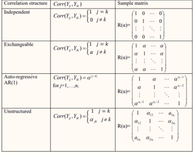
In Generalized Estimating Equations (GEE) models, correlation structures (Fig. 1) specify the relationship between observations within clusters, such as repeated measures on the same individuals or measurements from subjects within the same group. Choosing an appropriate correlation structure is essential for accurately modeling the dependencies in the data. Here’s a brief overview of common correlation structures used in GEE models:
-
Exchangeable: This is one of the simplest correlation structures, assuming that all pairs of observations within a cluster have the same correlation. It implies that the correlations between any two measurements within a cluster are equal. This structure is often used when there is no prior knowledge about the specific correlation pattern.
-
Independence: In this structure, it is assumed that all observations within a cluster are uncorrelated. This implies that there is no within-cluster correlation, making it suitable for data where observations within clusters are expected to be independent.
-
Autoregressive (AR): In this structure, the correlation between observations decreases as the time lag between them increases. It assumes that observations that are closer in time are more highly correlated than those farther apart. AR structures are commonly used for longitudinal data where observations are collected at equally spaced time intervals.
-
Unstructured: This structure allows for arbitrary correlations between all pairs of observations within a cluster. It provides the most flexibility but requires estimating a large number of parameters, making it less efficient when the number of clusters is small or the data are sparse.
-
Stationary: This structure assumes that the correlation between observations depends only on the time lag between them, not on the specific time points. It is a variation of the AR structure and is appropriate when the correlation pattern remains consistent over time.
-
Compound Symmetry (CS): Also known as the compound symmetry structure, it assumes constant correlation between all pairs of observations within a cluster, as well as constant variances for each variable. This structure is a combination of the exchangeable and autoregressive structures.
Choosing the appropriate correlation structure depends on the nature of the data and the underlying assumptions about the correlation pattern. Researchers often use model diagnostics, such as residual plots and goodness-of-fit tests, to assess the adequacy of the chosen correlation structure. Additionally, sensitivity analyses may be performed by comparing results across different correlation structures to ensure the robustness of the conclusions drawn from the GEE model.

Quasi-Likelihood under the Independence Model Criterion (QIC)
The Quasi-Likelihood under the Independence Model Criterion (QIC) is a goodness-of-fit measure used in the context of Generalized Estimating Equations (GEE) models. It serves as a criterion for model selection and comparison in situations where traditional likelihood-based measures may not be appropriate due to the complexity of the correlation structure.
Purpose
- Model Selection: QIC helps in selecting the best-fitting model among a set of candidate GEE models with different specifications of fixed effects, covariates, and correlation structures.
Calculation
-
Quasi-Likelihood: QIC is based on the quasi-likelihood function, which is an approximation to the likelihood function in GEE models. Quasi-likelihood is obtained by replacing the unknown correlation structure with an assumed working correlation structure.
-
Under Independence Model: QIC is calculated under the assumption of independence, where the working correlation structure is set to independence. This is often denoted as QICu (QIC under the independence model).
-
Penalization for Complexity: QIC incorporates a penalty term for model complexity, typically based on the number of parameters estimated in the model. This penalty term helps prevent overfitting by favoring simpler models.
-
Lower Values Indicate Better Fit: Like other information criteria (e.g., AIC, BIC), lower values of QIC indicate better model fit.
Interpretation
- Model Comparison: Researchers compare the QIC values of different models and select the model with the lowest QIC as the best-fitting model.
Limitations
-
Asymptotic Property: QIC is based on the quasi-likelihood function, which relies on asymptotic properties. Therefore, it may not perform optimally in small-sample situations.
-
Sensitivity to Model Assumptions: QIC is sensitive to assumptions about the working correlation structure. Choosing an inappropriate or misspecified working correlation structure can lead to biased QIC values.
-
Comparative Measure: QIC is most useful when comparing models rather than as an absolute measure of model fit. It should be used in conjunction with other diagnostic tools and criteria.
Practical Use
-
Software Implementation: Many statistical software packages that support GEE modeling provide facilities to compute QIC values automatically.
-
Model Refinement: Researchers often use QIC iteratively to refine models, starting with a simple model and gradually introducing complexity while monitoring changes in QIC.
Conclusion
The Quasi-Likelihood under the Independence Model Criterion (QIC) is a valuable tool for model selection and comparison in GEE modeling, providing a balance between goodness of fit and model complexity. However, it is essential to interpret QIC results in conjunction with other diagnostic tools and criteria and to be mindful of its limitations and assumptions.
An example of GEE model in R
# Install and load required package
install.packages("geepack")
library(geepack)

# Set seed for reproducibility
set.seed(123)

# Create simulated data
n <- 100  # Number of subjects
time_points <- 3  # Number of time points
time <- rep(1:time_points, each = n)
id <- rep(1:n, times = time_points)
group <- rep(c("Control", "Treatment"), each = n * time_points / 2)
covariate <- rnorm(n * time_points)
response <- 2 + 0.5 * covariate + rnorm(n * time_points)

# Create data frame
data <- data.frame(id, time, group, covariate, response)

# Perform GEE model with exchangeable correlation matrix
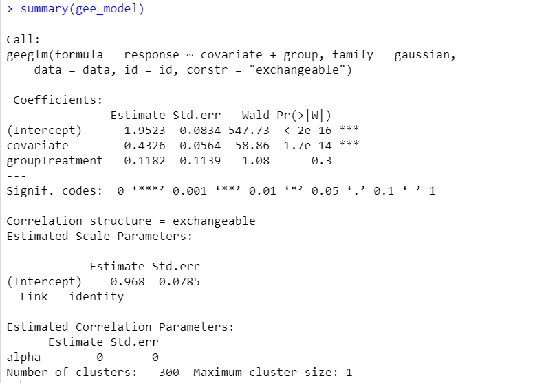
gee_model <- geeglm(response ~ covariate + group, id = id, data = data, family = gaussian, corstr = "exchangeable")

# Summary of the model
summary(gee_model)

Enjoy Reading This Article?
Here are some more articles you might like to read next: